

Wide Column Stores
Wide-column stores (Cassandra, HBase, ScyllaDB, Bigtable) store data in sparse, sorted, multi-dimensional maps: rows are keyed by a partition key, and within a partition, columns are sorted by a clustering key. They are optimized for massive write throughput (millions of writes/sec across a cluster) and time-series access patterns, at the cost of JOINs, ad-hoc queries, and strong cross-row consistency.
Foundational.
How it works
A wide-column store sits between a key-value store and a relational database. It is best understood as a sorted, sparse, multi-dimensional map: (row_key, column_key) → value, sorted by row key first, then by column key within a row.
Two implementations dominate:
- Google Bigtable (and its open-source cousins HBase, Accumulo) — the original. Rows are sorted lexicographically by row key; columns within a row are sorted and sparse (you only store columns you have data for).
- Apache Cassandra — derived from Amazon's Dynamo (distribution) and Bigtable (data model). Adds tunable consistency, peer-to-peer topology (no master), and a query language (CQL).
Both models share the same trade-off: they optimize for high write throughput and range scans within a partition, at the cost of JOINs, cross-row transactions, and ad-hoc queries.
ScyllaDB is a C++ rewrite of Cassandra that's wire-compatible (speaks CQL) but achieves 5-10× higher throughput per node by using a thread-per-core 'seastar' architecture instead of Cassandra's JVM.
The two most important decisions in wide-column schema design are:
- The partition key — determines which node holds the data. Hashed and distributed via consistent hashing across the cluster. All rows in a partition live on the same set of replica nodes and are queried together.
- The clustering key — sorts rows within a partition on disk. Range scans on the clustering key are sequential reads, the fastest possible disk pattern.
Get these right and a query like SELECT * FROM user_activity WHERE user_id = 42 AND activity_ts > '10:00' AND activity_ts < '11:00' is a single-partition lookup followed by a sequential on-disk read — O(log N + result size), with no fan-out across nodes.
Get them wrong and the query either fails outright (Cassandra refuses cross-partition range scans by default) or becomes a full-cluster scatter-gather that's 100× slower.
This is the fundamental mental shift from SQL: in Cassandra, the schema IS the query plan. You can't add an index later to fix a slow query — you'd have to design a new table that materializes the data in a different shape for that specific query. This pattern is called query-first design: enumerate the queries first, then create one table per query shape.
Every read and write in Cassandra specifies a consistency level: ONE, QUORUM, LOCAL_QUORUM, ALL, etc. With replication factor 3, QUORUM means 2 of 3 replicas must acknowledge. This gives you per-operation control of the latency/durability/consistency trade-off: ONE for fastest, QUORUM for strong-ish, ALL for strict (slowest, fails if any replica is down). The CAP-theorem math: reads + writes > replication factor → strong consistency (R+W>N). For RF=3: QUORUM reads + QUORUM writes = 2+2 > 3, so reads reflect all confirmed writes.
Wide-column stores are built on LSM trees (Log-Structured Merge trees), not B-trees. Writes go to an in-memory MemTable and an append-only commit log (for crash recovery); when the MemTable fills, it's flushed to disk as an immutable SSTable. Background compaction merges multiple SSTables into larger ones, discarding tombstones (deletion markers) and superseded versions.
The LSM architecture is the secret to Cassandra's write throughput: writes are always sequential appends, never random disk I/O. The cost is read amplification — a read may need to consult the MemTable plus multiple SSTables before finding the latest value (mitigated by Bloom filters and caches). It also means deletes are soft — tombstones persist until compaction, so heavy delete workloads can bloat disk usage and slow reads until compaction catches up.
This is the opposite trade-off from B-tree databases (PostgreSQL, MySQL), which optimize for fast point reads at the cost of slower random writes.
Use a wide-column store when:
- Write throughput is the bottleneck — millions of writes per second, beyond what a single SQL primary can handle.
- Time-series or event-log access patterns — data written in time order, queried by time range within an entity.
- Geo-distributed deployment — Cassandra's multi-datacenter replication is first-class (LOCAL_QUORUM keeps reads in-region).
- Schema is stable per query — you can enumerate queries up front and design tables for each.
- Eventual consistency is acceptable — telemetry, activity logs, messaging metadata.
Avoid wide-column stores when:
- You need ad-hoc analytical queries (use a columnar warehouse like ClickHouse, Snowflake, BigQuery).
- You need ACID transactions across rows (use SQL).
- Your access patterns are unknown or evolving fast (each new query shape needs a new table).
- The data is highly relational (use SQL or a graph DB).
- Read latency must be single-digit milliseconds with strong consistency (Cassandra is eventually consistent by default).
A useful rule of thumb: Cassandra is the right answer when you can describe every query as (partition_key, clustering_key_range) and accept that adding a new access pattern means writing a new materialized table.
You're storing IoT sensor data: 10,000 devices each emitting a reading every second, with queries like 'last 24 hours of readings for device X' and 'all readings for device X between time A and B'. What's the right Cassandra primary key, and why?
Pick one answer.
A teammate suggests adding an index on `device_id` to speed up a Cassandra query that filters by `reading_ts` only (no partition key). What's the right response?
Pick one answer.
Why does Cassandra achieve such high write throughput compared to a B-tree database like PostgreSQL?
Pick one answer.
Engineering mental model
Mental model. Think of Wide Column Stores as a deliberate boundary in a system. The boundary exists because something becomes harder to manage when everything is done in one place: latency, scale, failure isolation, consistency, cost, or team ownership. The useful question is not “what does Wide Column Stores mean?” but “what pressure makes this boundary worth introducing, and what new failure mode does it create?”
Before choosing Wide Column Stores, name the workload, the critical user path, the dominant bottleneck, the failure you are trying to absorb, and the trade-off you are willing to accept. If you cannot name those five things, the design is probably premature.
SELECT id, created_at
FROM records
WHERE tenant_id = ?
ORDER BY created_at DESC
LIMIT 50;

-- Ask: which index makes this query predictable at scale?Back-of-the-envelope reasoning
Numerical lens: write down traffic, payload size, read/write ratio, peak multiplier and durability target before choosing a component. The numbers should justify the architecture.
Interactive sandbox: Wide Column Stores
Wide-column stores optimize sparse reads. Predict disk seek cost for Wide Column Stores.
Change one variable at a time. Predict the failure mode first, then move the slider and see whether your mental model matches the simplified system response.
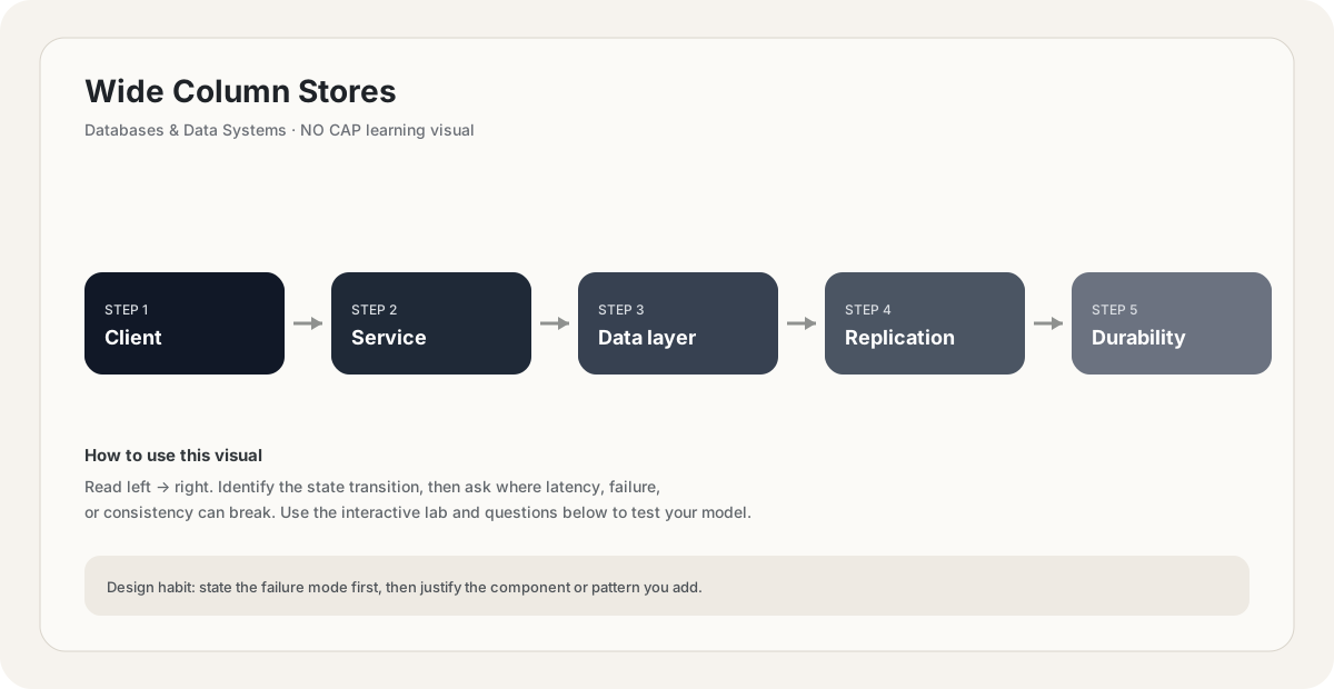
If you are stuck on Wide Column Stores, start by drawing the request path and marking every network hop, stateful component, queue, cache and failure boundary. Then estimate where the system will saturate.
You increase traffic by 10× in a system using Wide Column Stores. What should you inspect first?
Pick one answer.
Which statement is the safest engineering habit when using Wide Column Stores?
Pick one answer.
You have dashboards for traffic, latency, errors and saturation. You can change the architecture, but every change has operational cost.
Production scenario: your system uses Wide Column Stores, traffic suddenly spikes, and p99 latency doubles. What is your first move?
Interview drill
Answer this without notes: When would you choose Wide Column Stores, and when would you intentionally avoid it? Mention at least one bottleneck it addresses, one failure mode it introduces, and one alternative. Then quantify the workload you are designing for.
For Wide Column Stores, start with access patterns rather than brand names. Identify the dominant reads/writes, data relationships, consistency requirements, partition key, hot keys and failure behavior before choosing a storage strategy.
Numerical sanity check
A rough capacity check: required write throughput ≈ peak writes/s × average record size. At 5,000 writes/s and 2 KB average payloads, the raw incoming data stream is about 10 MB/s before indexes, replication and overhead.
Do not optimize for a memorized definition. Reason from the workload and failure mode.
A team proposes Wide Column Stores because it 'scales'. What workload characteristic would make that choice a poor fit?
Pick one answer.
What you gain, what you pay
- +Highest write throughput of any data model — millions of writes/sec per cluster.
- +Linear horizontal scalability — add nodes, redistribute ranges automatically.
- +First-class multi-datacenter replication — geo-distributed workloads are native.
- +Tunable consistency per operation — ONE, QUORUM, LOCAL_QUORUM, ALL.
- +Sequential on-disk writes (LSM) are durable-friendly and SSD-friendly.
- +Time-series access patterns are O(log N + result size) when partitioned correctly.
- −No JOINs — relationships must be denormalized or handled in app code.
- −No ad-hoc queries — every query shape needs its own table.
- −Eventual consistency by default — strong consistency (QUORUM+QUORUM) is slower.
- −Schema changes that alter partitioning require full table rebuilds.
- −Read amplification and tombstone bloat can hurt reads until compaction catches up.
- −Operational complexity — compaction strategy, repair, gc_grace_seconds all need tuning.
How this breaks in production
- Hot partition — bad partition key (timestamp, auto-increment) sends all writes to one node.
- Tombstone explosion — heavy deletes create many tombstones that slow reads until compaction.
- Unbounded partition growth — a partition key with too many clustering rows can exceed manageable size.
- Cross-partition range scans — accidentally querying without a partition key causes full-cluster scatter-gather.
- Stale data after read-repair lag — read-repair async writes can momentarily expose inconsistent data.
- Compaction storms — too-small compaction windows or bad strategy can saturate I/O and starve reads.
Don't fall into these traps
- •Designing tables like SQL — one big 'events' table and hoping indexes will fix queries.
- •Using a timestamp as the partition key — guarantees hot partitions and uneven load.
- •Forgetting that secondary indexes in Cassandra are not like SQL indexes — they're for narrow lookups, not range scans.
- •Treating Cassandra as strongly consistent by default — it isn't, and that's bitten many teams.
- •Not planning compaction strategy (SizeTiered vs Leveled vs TimeWindow) for the workload.
- •Not modeling materialized tables for each query shape — leading to slow cross-partition reads.
Real systems using this
How real systems implement this
- Netflix — Runs hundreds of Cassandra nodes across multiple AWS regions for viewing history, where every play event is appended and queried by user-time range. Uses LOCAL_QUORUM reads in-region to keep latency low while preserving consistency within a region.
- Discord — Originally stored billions of messages in Cassandra; moved to ScyllaDB (C++ rewrite of Cassandra, CQL-compatible) to reduce per-node overhead and the number of nodes needed. Their blog post on the migration is a classic case study in wide-column store tuning.
- Apple — Reported to run one of the largest Cassandra deployments in the world (tens of thousands of nodes) for Siri analytics and metrics — write-heavy, eventually consistent, time-bucketed queries.
- Instagram — Uses Cassandra for direct-message inbox storage — every message is keyed by recipient ID and timestamp, and reads are time-range scans within a partition.
Practice saying it out loud
- Q1When would you choose Cassandra over PostgreSQL? Over MongoDB? Over DynamoDB?
- Q2Design a Cassandra schema for storing user activity events with queries by user-time-range and by device-time-range. How many tables do you need?
- Q3Your Cassandra cluster is showing read latency spikes. Walk through what you'd investigate.
- Q4Explain the LSM tree vs B-tree trade-off and why it matters for write-heavy workloads.
- Q5What does `QUORUM` consistency mean in Cassandra with replication factor 3? What's the CAP-theorem implication of using QUORUM for both reads and writes?
Further reading & references
Core explanations are original NO CAP material. External references are provided for deeper study and standards.
What next?
Mark as understood once the mental model clicks.
Next recommended
Key-Value Stores